Over the past week, we have investigated several questions about draft pick valuation using our CP2 metric. First, we evaluated the Day 1 draft trades and found that teams trading down sometimes netted a substantial gain in overall draft stock. Next, we looked at where the real value in the draft lies and found that Day 2 draft pick value outpaces the first and third days. Finally, we asked whether the conventional wisdom is correct in asserting that it is a good idea to grab a quarterback early in the draft. Being a huge college football fan, I think it would be interesting to take a step back in time from the draft and turn our focus on the college programs producing these prospects in the first place.
In the college football landscape, it might seem a natural division to look at schools from the five power conferences versus non-power conference schools. However, there are problems with this way of looking at things, the biggest being that the power conferences often contain at least a few perennial bottom dwellers that produce little to no viable NFL prospects. Thus, instead of focusing on power conferences in their entirety, I will instead investigate power versus non-power schools individually.
Of course, this creates the problem of defining a “power school.” In the following analysis, I will use a definition of a power school suited to our present need; that is, those schools which produce the most draft picks. As we have discussed several times prior, the data on which we base our models runs from 2005 through the 2011 draft class, a total of seven years. For that reason, I will use a cutoff of four picks per year (28 total). This cutoff is admittedly somewhat arbitrary, and it excludes traditional power programs such as Michigan, Penn State, and Tennessee, each of whom produced a total of 26 draft picks from 2005-2011. But for the sake of a arriving at a round number it will suit us fine. This leaves us with 16 schools: Clemson, Florida State, Miami (FL), Virginia Tech, Iowa, Nebraska, Ohio State, Wisconsin, Texas, Oklahoma, USC, Alabama, Auburn, Florida, Georgia, and LSU. From 2005-2011, there were a total of 1782 draft picks, 548 (about 30%) of which came from one of these 16 “power schools.” Our main question then becomes: all else being equal, does it pay to draft a player from one of these power schools over a player from a non-power school?
We can first investigate this question graphically by using a plot of expected CP2 versus draft pick for the two groups. In each case, the curve is found by a non-linear regression using an exponential fitting function 
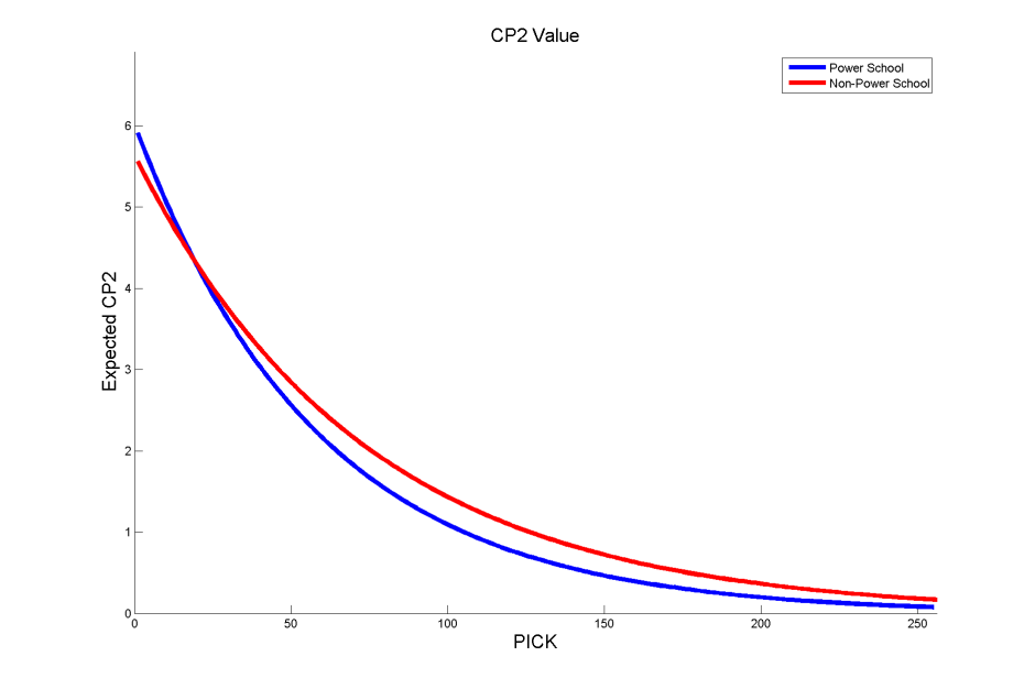
As we see, power school players are more valuable at the very top of the draft, but become less valuable near the end of the first round. Now, we might be tempted to conclude that non-power school players are more valuable in the aggregate, but a simple regression such as this cannot possibly be telling the whole story.
In order to see how inconclusive the first regression is, we turn to a parametric regression using LOWESS (locally weighted scatterplot smoothing). This type of regression uses local smoothing of the data by using a smoothing parameter (ranging from 0 to 1) to set the proportion of data used to perform this smoothing. In the following local regression, I use a minimal smoothing parameter (between 0.2 and 0.25) which preserves decreasing pick value.
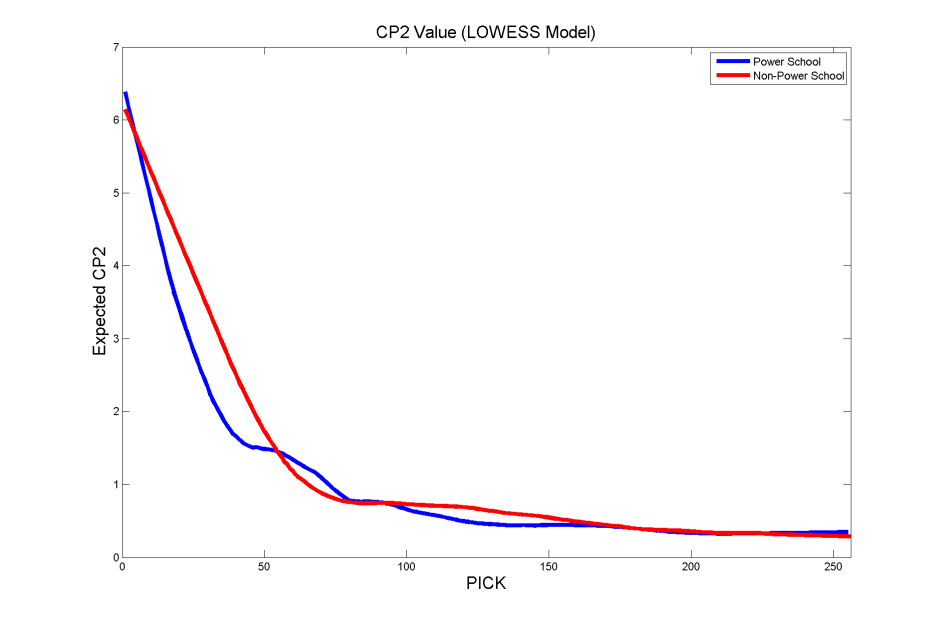
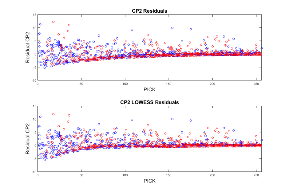
With the LOWESS model, we see the value of power school players is higher at only the very front end of the draft. After that, there seems to be a steep decline, but from the above plot we cannot honestly discern which group has more value because the fitting curves cross each other several times. In order to faithfully assess both models, we look to the residuals 
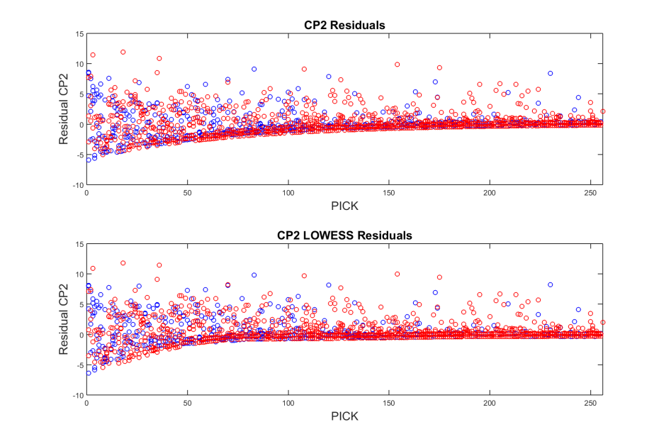
In the top plot, we find that the average residual for power schools is 0.120 and for non-power schools is 0.084. This difference is not statistically significant, but we get a feeling for what is going on by examining the plot itself. If we look closely, we see that at the end of the first round the negative residuals for the non-power school model are slightly larger than those of the power school model. This means that the non-power school model does not do quite as good of a job at predicting the actual data.
In the second plot, the average residual for the power school model is again larger than that of the non-power school model. We can also see from this plot that the negative residuals for the non-power school model show that it’s predictions generally overestimate the data from the first round through the second when compared to the model for power schools.
Overall, these results indicate there is no conclusive advantage in drafting players from power schools. Nevertheless, both models agree that non-power school players tend to be a more valuable pick beginning at the tail end of the first round and continuing through the second round, as well as in the fourth round. One possible explanation for this is that power school players are valued higher than they should be because of the national exposure that comes with playing for a premier program. It it worth noting that this difference would not be statistically significant if one were to throw 95% confidence intervals on the fitting curves, but the draft is all about gambling using every edge you can, perceived or real, and is the sort of scenario in which this kind of agreement between models can’t be ignored.
One final question we might ask is “How do non-power schools from the five power conferences stack up against the pool of non-power conference schools?” We again turn to a standard non-linear regression.
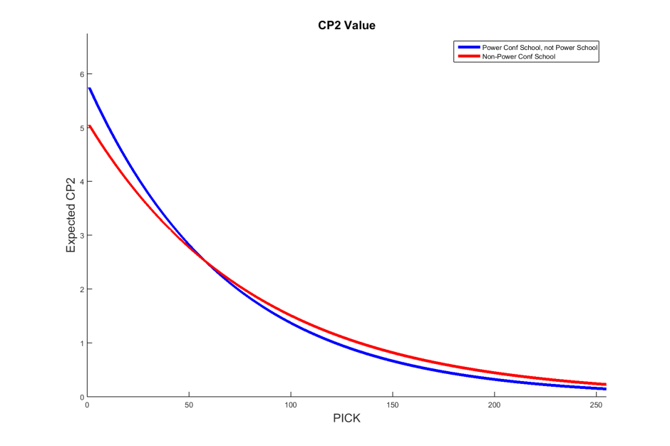
We see that power conference schools which do not qualify as power schools seem to produce more draft pick value up until the end of the second round. To investigate this further, we use LOWESS to generate a parametric regression (using a smoothing parameter of 0.25).

From the LOWESS model, we see that whatever differences we may have found in the exponential regression model could be seen as non-uniformity in the residuals. This plot shows that the two groups are very similar. We see this similarity echoed in the residual plots for each model.
We find there may be some slight overvaluing of early picks in the standard exponential model for power conference, non-power schools. The residuals for the LOWESS model appear to be well in line, suggesting that these two data sets are indeed very similar. Thus, it appears there is no meaningful difference in draft pick value between players from non-power schools in power conferences and players from those schools in non-power conferences.
In summary, we have seen that there is no statistically significant difference in draft value between players from power schools versus non-power schools, and the same analysis holds for non-power schools in power conferences versus non-power conference schools. An athlete surely gains national exposure by playing for a power school, but that exposure may only be useful for future marketing if he actually pans out in the NFL. I believe the data presented here shows that the detailed work of NFL scouts–along with the arduous combine and pro day process–ensure that pro teams form a complete picture of a player that does not rely on what school they attended.
